Part 1 Introduction

1.1 Getting Started

1.1.1 Why R

• Dedicated to statistics
• very powerful language for data science / data analysis
• Easy plotting and mapping (compared to Python)
• Strong algorithms for spatial analysis and spatial statistics
• Easy reporting with Rmarkdown

1.1.2 Why Rstudio

• R dedicated IDE
• compatible with Rmarkdown (comes with pandoc)
• R oriented addins

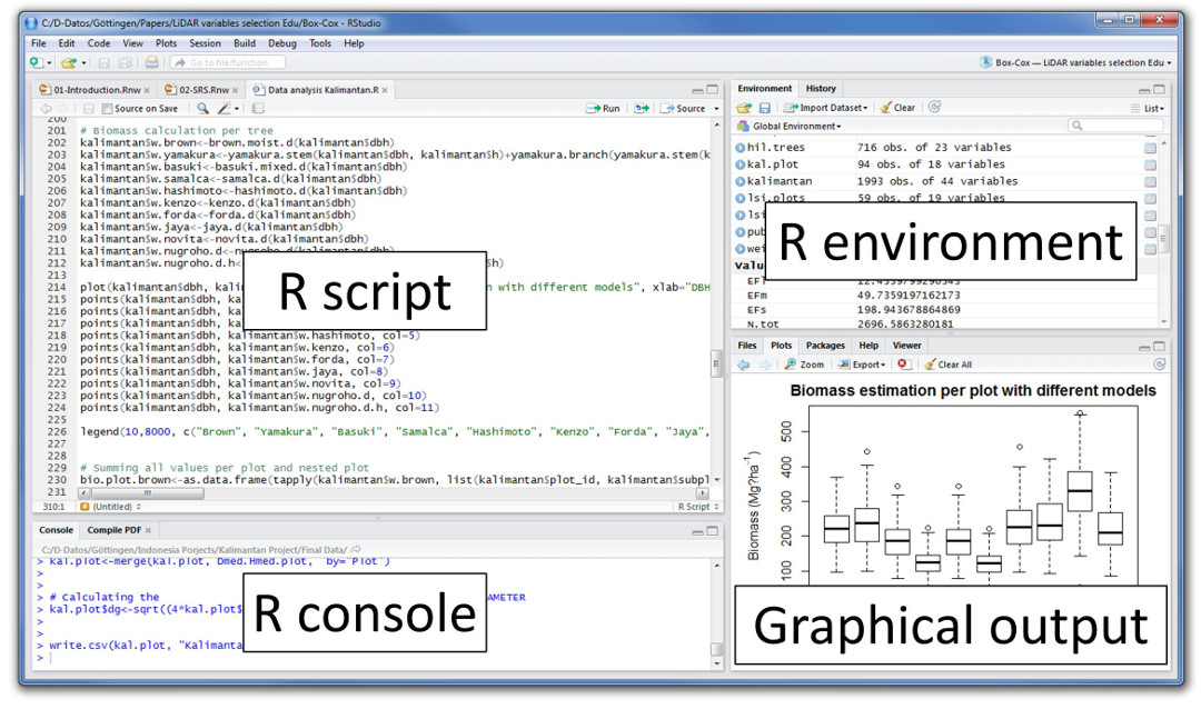
Rstudio interface (image source)

1.1.3 Why using the Tidyverse

• packages set for R
• aimed to data analysis
• homogenous
• compatible with R base and other paradigms

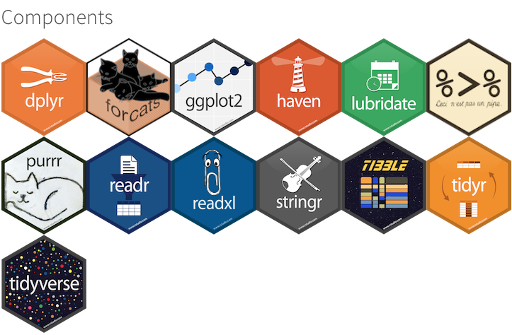
Tidyverse packages

1.2 Rmarkdown

Rmarkdown is a markup language aiming to produce high quality document with the lightest syntax possible. You can mix code (R, Python, bash, etc) within the text.

The code will be evaluated at the document compilation.

With the same Rmarkdown file you can generate different formats like HTML, PDF and Epub.

Several templates are provided (reports, books, slideshow) that you can personalise.

1.2.1 Basic workflow

• write text and code
• compile
• get a document (html, pdf, etc)

1.2.2 Rmarkdown basics

1.2.2.1 Create an empty document from a template

• create a new Rmardown document (.Rmd)
• Choose a title and write the author name
• Select a template (HTML is fine)
• press OK

1.2.2.2 Fill the yaml header

title: "R basics"
author: "Nicolas Roelandt"
date: "2019/01/14"
output: html_document

• Set options if needed
• Write your content

1.2.2.3 Exports

• HTML file
• PDF report (needs LaTeX or {tinyTeX})
• Word document
• Presentations

knit document to render

1.2.2.4 Text formatting

1.2.2.4.1 Headers

# Level 1 header
## Level 2 header
...
##### Level 5 header

1.2.2.4.2 Markup

- *italic*
- _italic_
- **bold**
- __bold__

1.2.2.4.3 Add illustrations

![pic description](pic url)

1.2.2.4.4 Ordered list

1. First thing
2. Second thing
4. Third thing
3. Fourth thing

1. First thing
2. Second thing
3. Third thing
4. Fourth thing

1.2.2.4.5 An unordered list

- this is one thing
- this is another, this next part is **important**
+ this is a bit of `inline code`
+ this is a [link](https://roelandtn.frama.io)

• this is one thing
• this is another, this next part is important
• this is a bit of inline code
• this is a link

1.3 Code cells

This is a R code cell:

```r
## Put your code  (this is a commented line btw) 
```

1.3.0.0.1 Code cells

This is a code cell

```r
library(ggplot2)    
ggplot(mtcars) +    
  aes(mpg, disp) +  
  geom_point() +    
  geom_smooth()     
```

You can write code in it and execute it !

• cell by cell (green arrow on the top right of the cell);
• with the Run menu;
• highlight a code line and press Ctrl + enter to execute only the selected lines.

Time to write some code !

1.4 R basics

1.4.1 Mathematical operations

Write one by one those commands in the Rstudio console:

3 + 2
8 - 4
7 * 3
7 / 3 

Now write in 4 cells of your Rmarkdown document and run them.

Do you see a difference ?

And if you put them in the same cell ?

1.4.2 Data types

• numeric:
  • 2
  • 12.125
• character strings: “a”, “word”
• logical:
  • TRUE
  • FALSE
  • NULL (sort of)

Please note that logicals are in capital letters.

• vectors:
• a <- c(12, 15, 35698)
• list: list(1, 45, 12.0, "toto")
• matrices : matrix(0:9, 3,3)
• dataframe (df) : data.frame(x = 1:3, y = c('a', 'b', 'c'))
• constants:
  • letters[3:4]
  • LETTERS[12:26]
  • pi

Vector are a collection of object of same type. If you mix numeric and strings, it will become all strings You can mix types in list

1.4.3 Comparison and logical operators

1 > 4 # FALSE

## [1] FALSE

3 < 5 # TRUE

## [1] TRUE

3 >= 2 # TRUE

## [1] TRUE

4 <= 1 # FALSE

## [1] FALSE

1 >  2 & 3 > 2 # FALSE AND TRUE => FALSE

## [1] FALSE

1 >  2 | 3 > 2 # FALSE OR TRUE => TRUE

## [1] TRUE

1.4.4 Affectation

• keep data in memory
• use variables
• use <- (or =)

Examples:

a <- c(0:9) # new integer vector
c <- list(1, 45, 12.0, "toto")
d <- matrix(0:9, 3,3)

## Warning in matrix(0:9, 3, 3): la longueur des données [10] n'est pas un
## diviseur ni un multiple du nombre de lignes [3]

1.4.5 not only a calculator

• R is shipped with lots of functions:

data(<datasetname>)   # load an embedded dataset
head(<objectname)     # first lines of a dataframe
is.vector(object)     # return TRUE if object is a vector
is.data.frame(object) # return TRUE if object is a data.frame
typeof(<objectname)   # Type of an object
getwd()               # get the current working directory
setwd(<PATH>)         # set new working directory 
rm()                  # remove a object from memory
unique()              # returns unique values

• Try to load the mtcars dataset,
• type head(mtcars)
• get the type of 12, 14.6, TRUE

1.4.5.1 Write functions

##### Why ?

Because core functions does not covers all need, you might need specific functions. Expecially if you want to reuse code.

1.4.5.1.1 When ?

When you have to copy past code more than twice.

DRY: Don’t Repeat Yourself

1.4.5.1.2 Syntax

<function name> <- function (arguments){
  # function body
  # last statement will be returned by default
}

1.4.5.1.3 Example

square <- function (x){
  x_square <- x**2
  x_square
  #return(x_square) # explicit return
}

square(3) # call of the function with 3 as a parameter

## [1] 9

1.5 Get help

Help in the R language is very well documented. To be published on the CRAN repository, all the functions of a package needs to be documented. This documentation should give information on parameters and output, the options and provide working examples.

You can call the help function with a question mark.

help(<functionname>)
?<functionname>

# example
help(mean)
?summary

1.6 Packages management

• R comes with core functions
• It can be extended with packages
• Packages can downloaded from repos like CRAN (The Comprehensive R Archive Network) or others sources.

1.6.1 Install packages

With the command install.packages(<package name>)

1.6.2 Load packages

With the command library(<package name>)

1.6.3 Exercice

Try to install and load the package skimr

(If it doesn’t work because of internet, it is ok)

install.packages() will install the packages the first time on the computer.

library() will load an installed package. You have to run it in every script that use functions from this package.

Good practice is to load packages at the beginning of the script so if a package is missing, you’ll get the error from the beginning.

1.6.4 Write packages

You can write your own packages for

• reusability
• easier maintenance
• thematic grouping

It is not the point of this course, for more informations look at Hadley Wickham’s R packages book