Part 2 Data manipulation with R

2.1 Get Started

Multiple choices cases

R base
Tidyverse
datatable

2.2 Data wrangling with R base

2.2.1 Load data

2.2.1.1 Load data from an embedded data set:

LakeHuron <- LakeHuron : loads explicitly the Lake Huron dataset
Look at the Environnement panel
type LakeHuron

This can be useful to reproduce documentation examples but it is not your data. You need to load data from the outside.

2.2.1.2 Load data from a csv file

worldbank <- read.csv("data/worldbank_df.csv", sep = ',', header = TRUE)

"data/worldbank_df.csv" is the path to the file, from the working directory. Note that, even on Microsoft Windows, path notation use slashes / to separate directories.

sep* and header are options to set accordingly to your file.

This would have work too:

worldbank <- read.csv("data/worldbank_df.csv")

2.2.1.3 What’s the difference between LakeHuron and worldbank ?

Tips : - Look into the Environnement panel - use the class function

`LakeHuron ̀is a time series, there is just one column with the water height. But the start and ending years are indicated

̀worldbank_df ̀ is a dataframe with several columns (name, urban pop)

2.2.2 Get some insight about the data

2.2.2.1 Dataset dimensions

length(): to get the length of a vector

length(LakeHuron)

## [1] 98

There is 98 records in the LakeHuron dataset.

nrow()̀̀ : number of rows of a dataset

nrow(worldbank)

## [1] 177

There is 177 rows in the worldbank dataset.

dim() : dimensions (number of rows and columns) of a dataset

dim(worldbank) # returns a vector :  [1] is the number of rows, [2] the number of columns

## [1] 177   7

There is 177 rows and 7 columns in the dataset.

2.2.2.2 Descriptives statistics

Mean

mean(LakeHuron)

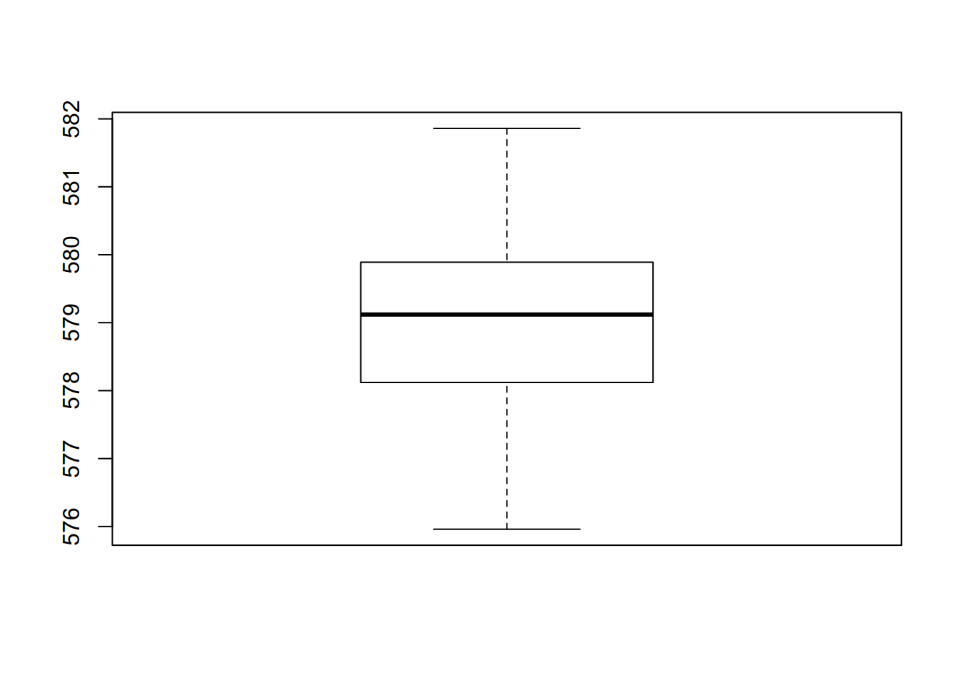
## [1] 579.0041

Median

median(LakeHuron)

## [1] 579.12

Minimum

min(LakeHuron)

## [1] 575.96

Maximum

max(LakeHuron)

## [1] 581.86

Range

range(LakeHuron)

## [1] 575.96 581.86

Quantiles

quantile(LakeHuron)

##      0%     25%     50%     75%    100% 
## 575.960 578.135 579.120 579.875 581.860

Variance

var(LakeHuron, na.rm = TRUE)

## [1] 1.737911

Standard deviation

sd(LakeHuron, na.rm = TRUE)

## [1] 1.318299

Summary

summary(LakeHuron, na.rm = TRUE)

##    Min. 1st Qu.  Median    Mean 3rd Qu.    Max. 
##   576.0   578.1   579.1   579.0   579.9   581.9

The na.rm = TRUE option remove the Non Available data before computation in order to avoid taking it in account as zeros.

2.2.2.3 Work with columns

2.2.2.3.1 How to get the column names ?

names(worldbank)

## [1] "name"         "iso_a2"       "HDI"          "urban_pop"   
## [5] "unemployment" "pop_growth"   "literacy"

##### Get the content of a column

as an object

head(worldbank$name)

## [1] Afghanistan          Angola               Albania             
## [4] United Arab Emirates Argentina            Armenia             
## 177 Levels: Afghanistan Albania Algeria Angola Antarctica ... Zimbabwe

The head() function display only the 6 first rows, what does the tail() function ?

By column name

head(worldbank$name)

# is equivalent to
head(worldbank["name"])

##                   name
## 1          Afghanistan
## 2               Angola
## 3              Albania
## 4 United Arab Emirates
## 5            Argentina
## 6              Armenia

By column order

head(worldbank$name)
head(worldbank["name"])

head(worldbank[,1])

## [1] Afghanistan          Angola               Albania             
## [4] United Arab Emirates Argentina            Armenia             
## 177 Levels: Afghanistan Albania Algeria Angola Antarctica ... Zimbabwe

In brackets first digits are the row numbers, after the comma it is the column numbers.

2.2.2.3.2 Slicing

Syntax : Numbers between brackets: [2:3]

Create an example vector a

a <- c(1:10)
a

##  [1]  1  2  3  4  5  6  7  8  9 10

Slice the a vector

a[2:5]

## [1] 2 3 4 5

Slicing works with columns

Numbers between brackets: [<rows> , <columns>]

d <- matrix(1:9, 3, 3) # 3 by 3 matrices with number from 1 to 9

Only the columns 2 and 3

d[,2:3]

##      [,1] [,2]
## [1,]    4    7
## [2,]    5    8
## [3,]    6    9

Just the first row of the columns 2 and 3

d[3,2:3]

## [1] 6 9

What is that code doing ?

worldbank[1:6,1]

worldbank[1:6,1]

## [1] Afghanistan          Angola               Albania             
## [4] United Arab Emirates Argentina            Armenia             
## 177 Levels: Afghanistan Albania Algeria Angola Antarctica ... Zimbabwe

2.2.2.3.2.1 Exercice

Try to get the 10 first rows and the 3 first columns of the worldbank dataset.

##                                   name iso_a2   HDI
## 1                          Afghanistan     AF    NA
## 2                               Angola     AO 0.504
## 3                              Albania     AL    NA
## 4                 United Arab Emirates     AE    NA
## 5                            Argentina     AR    NA
## 6                              Armenia     AM    NA
## 7                           Antarctica     AQ    NA
## 8  French Southern and Antarctic Lands     TF    NA
## 9                            Australia     AU    NA
## 10                             Austria     AT    NA

worldbank[1:10,1:3]

##                                   name iso_a2   HDI
## 1                          Afghanistan     AF    NA
## 2                               Angola     AO 0.504
## 3                              Albania     AL    NA
## 4                 United Arab Emirates     AE    NA
## 5                            Argentina     AR    NA
## 6                              Armenia     AM    NA
## 7                           Antarctica     AQ    NA
## 8  French Southern and Antarctic Lands     TF    NA
## 9                            Australia     AU    NA
## 10                             Austria     AT    NA

For more precision on slicing, use vectors:

worldbank[c(1,3,5),c(1,4)]

##          name urban_pop
## 1 Afghanistan   8609463
## 3     Albania   1629715
## 5   Argentina  39372787

# or
worldbank[seq(1,5,2),c("name","urban_pop")]

##          name urban_pop
## 1 Afghanistan   8609463
## 3     Albania   1629715
## 5   Argentina  39372787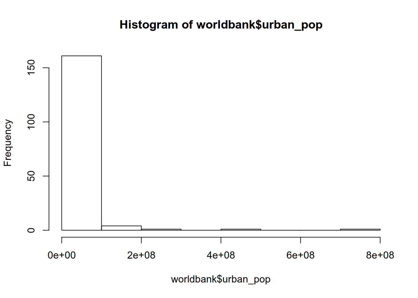

2.2.3 Plots

2.2.3.1 Histograms

hist(worldbank$urban_pop)

You can modify some parameters :

hist(worldbank$urban_pop, 
     main = "Urban population", # plot title
     xlab= "Urban population")  # X axis label

2.2.3.2 Boxplot

boxplot(LakeHuron)

2.2.3.3 Scatterplot

2.3 Data wrangling with the Tidyverse

2.3.1 First load the tidyverse package

library(tidyverse)

## ── Attaching packages ────────────────────────────────── tidyverse 1.3.0 ──

## ✔ ggplot2 3.2.1     ✔ purrr   0.3.3
## ✔ tibble  2.1.3     ✔ dplyr   0.8.3
## ✔ tidyr   1.0.0     ✔ stringr 1.4.0
## ✔ readr   1.3.1     ✔ forcats 0.4.0

## ── Conflicts ───────────────────────────────────── tidyverse_conflicts() ──
## ✖ dplyr::filter() masks stats::filter()
## ✖ dplyr::lag()    masks stats::lag()

Then ask questions

most useful tydiverse package for data manipulation is dplyr
each action is a verb
- filter – select a subset of the rows of a data frame
- arrange – works similarly to filter, except that instead of filtering or selecting rows, it reorders them
- select – select columns of a data frame
- mutate – add new columns to a data frame that are functions of existing columns
- summarize – summarize values
- group_by – describe how to break a data frame into groups of rows
you can pipe successive actions with a %>%
Tibbles: dataframes++

2.3.2 Dataset

We will use the gapminder dataset:

library(gapminder)
head(gapminder)

## # A tibble: 6 x 6
##   country     continent  year lifeExp      pop gdpPercap
##   <fct>       <fct>     <int>   <dbl>    <int>     <dbl>
## 1 Afghanistan Asia       1952    28.8  8425333      779.
## 2 Afghanistan Asia       1957    30.3  9240934      821.
## 3 Afghanistan Asia       1962    32.0 10267083      853.
## 4 Afghanistan Asia       1967    34.0 11537966      836.
## 5 Afghanistan Asia       1972    36.1 13079460      740.
## 6 Afghanistan Asia       1977    38.4 14880372      786.

The gapminder data frames include six variables, (Gapminder.org documentation page):

variable	meaning
country
continent
year
lifeExp	life expectancy at birth
pop	total population
gdpPercap	per-capita GDP

Per-capita GDP (Gross domestic product) is given in units of international dollars, “a hypothetical unit of currency that has the same purchasing power parity that the U.S. dollar had in the United States at a given point in time” – 2005, in this case.

gapminder: 12 rows for each country (1952, 1955, …, 2007).

2.3.3 select()

Select one or more column by name. Let’s keep only the year, country and gdpPercap columns.

year_country_gdp <- gapminder %>% 
    select(year, country, gdpPercap) 
year_country_gdp

## # A tibble: 1,704 x 3
##     year country     gdpPercap
##    <int> <fct>           <dbl>
##  1  1952 Afghanistan      779.
##  2  1957 Afghanistan      821.
##  3  1962 Afghanistan      853.
##  4  1967 Afghanistan      836.
##  5  1972 Afghanistan      740.
##  6  1977 Afghanistan      786.
##  7  1982 Afghanistan      978.
##  8  1987 Afghanistan      852.
##  9  1992 Afghanistan      649.
## 10  1997 Afghanistan      635.
## # … with 1,694 more rows

2.3.4 filter()

Filter rows matching a condition (TRUE or FALSE test). We will keep only records in Europe.

year_country_gdp_euro <- gapminder %>%
    filter(continent == "Europe") %>% 
    select(year, country, gdpPercap)
year_country_gdp_euro

## # A tibble: 360 x 3
##     year country gdpPercap
##    <int> <fct>       <dbl>
##  1  1952 Albania     1601.
##  2  1957 Albania     1942.
##  3  1962 Albania     2313.
##  4  1967 Albania     2760.
##  5  1972 Albania     3313.
##  6  1977 Albania     3533.
##  7  1982 Albania     3631.
##  8  1987 Albania     3739.
##  9  1992 Albania     2497.
## 10  1997 Albania     3193.
## # … with 350 more rows

Trick

If you want to know unique values to filter on, use the unique() function !

unique(gapminder["continent"])

## # A tibble: 5 x 1
##   continent
##   <fct>    
## 1 Asia     
## 2 Europe   
## 3 Africa   
## 4 Americas 
## 5 Oceania

Exercice 1

Produce a dataframe that has the African values for lifeExp, country and year, but not for other Continents

## # A tibble: 624 x 3
##     year country lifeExp
##    <int> <fct>     <dbl>
##  1  1952 Algeria    43.1
##  2  1957 Algeria    45.7
##  3  1962 Algeria    48.3
##  4  1967 Algeria    51.4
##  5  1972 Algeria    54.5
##  6  1977 Algeria    58.0
##  7  1982 Algeria    61.4
##  8  1987 Algeria    65.8
##  9  1992 Algeria    67.7
## 10  1997 Algeria    69.2
## # … with 614 more rows

Hint

year_country_lifeExp_Africa <- --------- %>%
      filter(continent == "------") %>%  
      select(year, ------ , -----)     
year_country_lifeExp_Africa

2.3.5 mutate()

mutate() allows to add new columns to a dataset. transmute() use the same syntax but only keep the new columns.

gapminder %>% 
  mutate( total_gdp = pop * gdpPercap
    )

## # A tibble: 1,704 x 7
##    country     continent  year lifeExp      pop gdpPercap    total_gdp
##    <fct>       <fct>     <int>   <dbl>    <int>     <dbl>        <dbl>
##  1 Afghanistan Asia       1952    28.8  8425333      779.  6567086330.
##  2 Afghanistan Asia       1957    30.3  9240934      821.  7585448670.
##  3 Afghanistan Asia       1962    32.0 10267083      853.  8758855797.
##  4 Afghanistan Asia       1967    34.0 11537966      836.  9648014150.
##  5 Afghanistan Asia       1972    36.1 13079460      740.  9678553274.
##  6 Afghanistan Asia       1977    38.4 14880372      786. 11697659231.
##  7 Afghanistan Asia       1982    39.9 12881816      978. 12598563401.
##  8 Afghanistan Asia       1987    40.8 13867957      852. 11820990309.
##  9 Afghanistan Asia       1992    41.7 16317921      649. 10595901589.
## 10 Afghanistan Asia       1997    41.8 22227415      635. 14121995875.
## # … with 1,694 more rows

Change mutate() by transmute() and compare the results.
How to keep the year and country column ?

2.3.6 group_by()

Group data by a variable.

str(gapminder)

## Classes 'tbl_df', 'tbl' and 'data.frame':    1704 obs. of  6 variables:
##  $ country  : Factor w/ 142 levels "Afghanistan",..: 1 1 1 1 1 1 1 1 1 1 ...
##  $ continent: Factor w/ 5 levels "Africa","Americas",..: 3 3 3 3 3 3 3 3 3 3 ...
##  $ year     : int  1952 1957 1962 1967 1972 1977 1982 1987 1992 1997 ...
##  $ lifeExp  : num  28.8 30.3 32 34 36.1 ...
##  $ pop      : int  8425333 9240934 10267083 11537966 13079460 14880372 12881816 13867957 16317921 22227415 ...
##  $ gdpPercap: num  779 821 853 836 740 ...

str(gapminder)

str(gapminder %>% group_by(continent))

## Classes 'tbl_df', 'tbl' and 'data.frame':    1704 obs. of  6 variables:
##  $ country  : Factor w/ 142 levels "Afghanistan",..: 1 1 1 1 1 1 1 1 1 1 ...
##  $ continent: Factor w/ 5 levels "Africa","Americas",..: 3 3 3 3 3 3 3 3 3 3 ...
##  $ year     : int  1952 1957 1962 1967 1972 1977 1982 1987 1992 1997 ...
##  $ lifeExp  : num  28.8 30.3 32 34 36.1 ...
##  $ pop      : int  8425333 9240934 10267083 11537966 13079460 14880372 12881816 13867957 16317921 22227415 ...
##  $ gdpPercap: num  779 821 853 836 740 ...

## Classes 'grouped_df', 'tbl_df', 'tbl' and 'data.frame':  1704 obs. of  6 variables:
##  $ country  : Factor w/ 142 levels "Afghanistan",..: 1 1 1 1 1 1 1 1 1 1 ...
##  $ continent: Factor w/ 5 levels "Africa","Americas",..: 3 3 3 3 3 3 3 3 3 3 ...
##  $ year     : int  1952 1957 1962 1967 1972 1977 1982 1987 1992 1997 ...
##  $ lifeExp  : num  28.8 30.3 32 34 36.1 ...
##  $ pop      : int  8425333 9240934 10267083 11537966 13079460 14880372 12881816 13867957 16317921 22227415 ...
##  $ gdpPercap: num  779 821 853 836 740 ...
##  - attr(*, "groups")=Classes 'tbl_df', 'tbl' and 'data.frame':   5 obs. of  2 variables:
##   ..$ continent: Factor w/ 5 levels "Africa","Americas",..: 1 2 3 4 5
##   ..$ .rows    :List of 5
##   .. ..$ : int  25 26 27 28 29 30 31 32 33 34 ...
##   .. ..$ : int  49 50 51 52 53 54 55 56 57 58 ...
##   .. ..$ : int  1 2 3 4 5 6 7 8 9 10 ...
##   .. ..$ : int  13 14 15 16 17 18 19 20 21 22 ...
##   .. ..$ : int  61 62 63 64 65 66 67 68 69 70 ...
##   ..- attr(*, ".drop")= logi TRUE

If you look at the grouped dataframe, you can see that group_by created new smaller dataframes (one by continent) along side the original one.

All following calculations within the summarize() function will be made on those separated dataframes.

2.3.7 summarize()

summarize() aggregates the grouped data with a function (sum, mean, custom, etc.).

gdp_bycontinents <- gapminder %>%
    group_by(continent) %>%
    summarize( 
      mean_gdpPercap=mean(gdpPercap) 
      ) 
gdp_bycontinents

## # A tibble: 5 x 2
##   continent mean_gdpPercap
##   <fct>              <dbl>
## 1 Africa             2194.
## 2 Americas           7136.
## 3 Asia               7902.
## 4 Europe            14469.
## 5 Oceania           18622.

]

Exercice 2

Calculate mean and median life expectancy in South Africa and Ireland

Steps

Select the columns
Filter the countries
summarize the data in 2 new variables

Expected output

## # A tibble: 1 x 2
##   AverageLife MedianLife
##         <dbl>      <dbl>
## 1        63.5       64.4

Hint

AverageLife <- gapminder %>%
    -----(country, -----) %>%       
    -------(---- == "South Africa" | 
             country == -----) %>% 
    --------( 
      AverageLife=mean(----), 
      MedianLife=median(lifeExp) 
      ) 
AverageLife

Exercice 3

Calculate the gap between a mean life expectancy in a country and the world mean life expectancy.

Steps

Select the columns
Create a new variable lifeExp_gap
Group data by country
Summarize by creating 2 new variables country_mean_life_exp and country_mean_life_exp_gap

Expected output

## # A tibble: 142 x 3
##    country     country_mean_life_exp country_mean_life_exp_gap
##    <fct>                       <dbl>                     <dbl>
##  1 Afghanistan                  37.5                   -22.0  
##  2 Albania                      68.4                     8.96 
##  3 Algeria                      59.0                    -0.444
##  4 Angola                       37.9                   -21.6  
##  5 Argentina                    69.1                     9.59 
##  6 Australia                    74.7                    15.2  
##  7 Austria                      73.1                    13.6  
##  8 Bahrain                      65.6                     6.13 
##  9 Bangladesh                   49.8                    -9.64 
## 10 Belgium                      73.6                    14.2  
## # … with 132 more rows

Hint

mean_lifeExp_gap <- ----- %>%
    ------(country, lifeExp) %>%
    -----( # creates a new column
      lifeExp_gap = lifeExp - mean(lifeExp)
      ) %>%
    -------(country) %>%
    summarize( 
      country_mean_life_exp = 
        ----(lifeExp), 
      country_mean_life_exp_gap = 
        ----(----) 
      )
mean_lifeExp_gap

2.3.7.1 Sort data

If needed you can arrange rows by life expectancy gaps.

Ascending order

mean_lifeExp_gap <- mean_lifeExp_gap %>%
    arrange(country_mean_life_exp_gap) 
head(mean_lifeExp_gap)

Descending order

mean_lifeExp_gap <- mean_lifeExp_gap %>%
    arrange(desc(country_mean_life_exp_gap)) 
head(mean_lifeExp_gap)

## # A tibble: 6 x 3
##   country       country_mean_life_exp country_mean_life_exp_gap
##   <fct>                         <dbl>                     <dbl>
## 1 Sierra Leone                   36.8                     -22.7
## 2 Afghanistan                    37.5                     -22.0
## 3 Angola                         37.9                     -21.6
## 4 Guinea-Bissau                  39.2                     -20.3
## 5 Mozambique                     40.4                     -19.1
## 6 Somalia                        41.0                     -18.5

## # A tibble: 6 x 3
##   country     country_mean_life_exp country_mean_life_exp_gap
##   <fct>                       <dbl>                     <dbl>
## 1 Iceland                      76.5                      17.0
## 2 Sweden                       76.2                      16.7
## 3 Norway                       75.8                      16.4
## 4 Netherlands                  75.6                      16.2
## 5 Switzerland                  75.6                      16.1
## 6 Canada                       74.9                      15.4

2.3.8 Commands order

Even not mandatory, it is recommended to use that order:

filter the rows
select the columns
mutate if needed
group by if needed
summarize if needed

filter and select first to reduce the size of the dataset to handle.
filter first to avoid issues by not selecting columns that are used to filter.

Now let’s see how to plot with ggplot2